Loom: Atlas view
We have just published the second phase of Loom which we are calling ‘Atlas’. See the second icon on Loom.

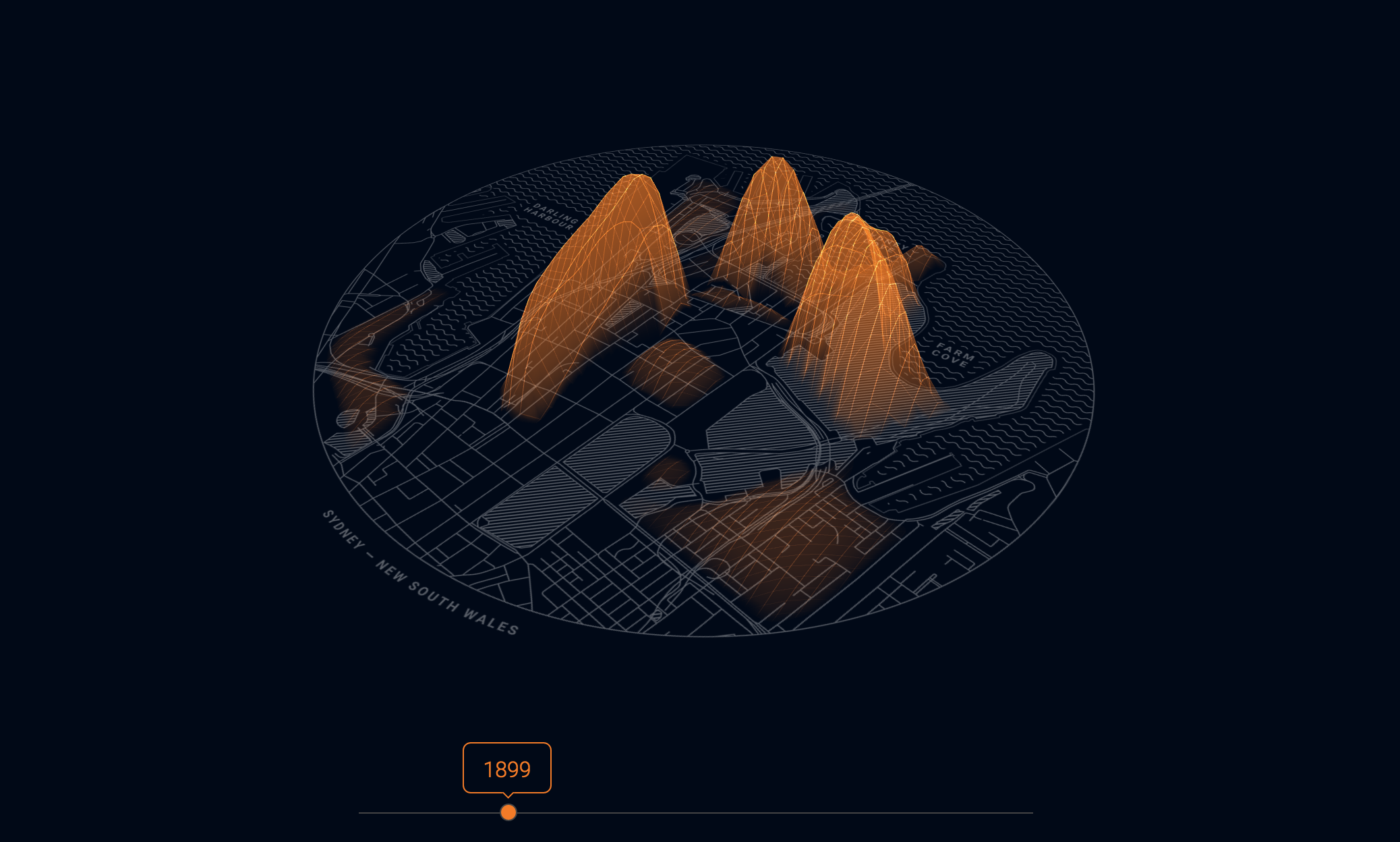
This is a heat map view of the same location data from the ‘looseleaf’ phase but we have provided 10 more specific areas within the CBD location for exploring.
These include:
- Circular Quay
- The Rocks
- Botanic Gardens
- Martin Place
- George Street
- Darling Harbour
- St Mary’s Cathedral
- Millers Point
- Woolloomooloo
- Bridge Street
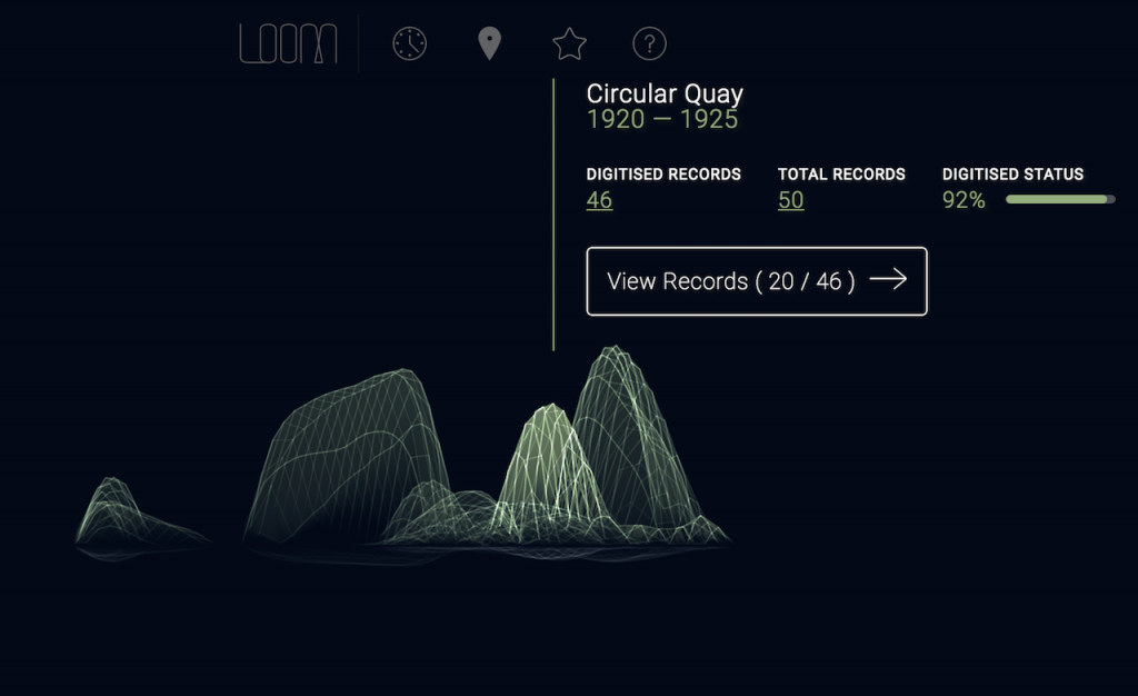
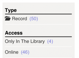
With this phase we are pulling in the data about what has been digitised in the selected areas according to time from 1870 to 2000. For example, if you click on the peak elevation for Circular Quay in the 20s you will get the result of 46 digitised records from 50 available records. The lower elevations represents items that are available ‘Only in the Library’ and this is linked to our catalogue so the items can be researched further.
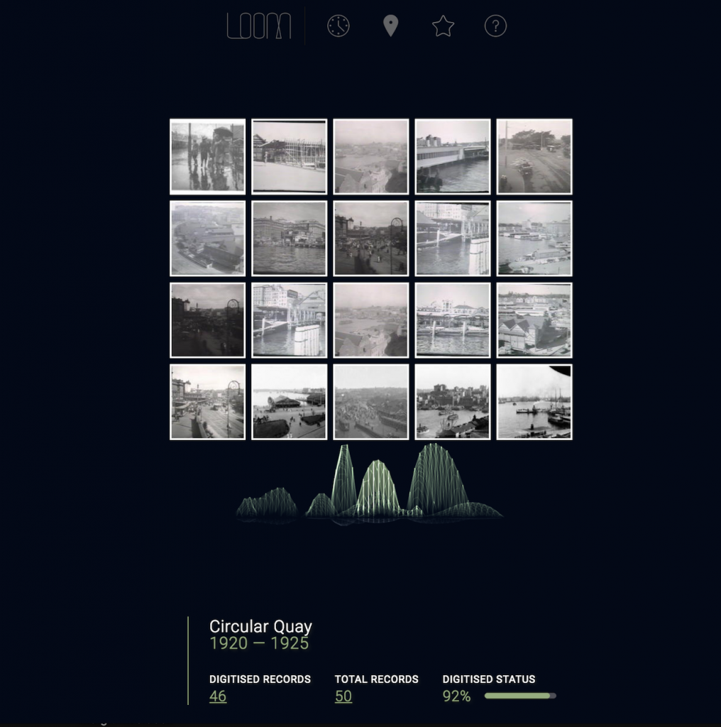
We decided to include a gallery view of the first 20 images for each return. We have added only the first 20 images at this stage for capacity reasons as we are working with a lot more data than in the first phase of Loom. There are now 3000 items instead of 300 and if we loaded all of the records it would slow down the experience and load time for the user. This will be one of the considerations we will take on board when we finish the three prototyping phases and move into a business as usual approach for the interface.
Technologies (from Grumpy Sailor)
- The site build is using http://yeoman.io
- The 3D visualisation uses WebGL (ThreeJS ) and all the UI elements are HTML.
- To collect and prepare the data from State Library Funnelback API we used Python scripts.
Atlas explores new ways of using WebGL to visualise data points on a map terrain.
Atlas uses Shaders to draw the map and manipulate all the vertices to animate the elevations, which when coupled with the data from the ACMS to show on the map, it becomes quite complex. From our research and findings there is very few current projects using Shaders with data as used in Atlas.
How the map elevations are calculated?
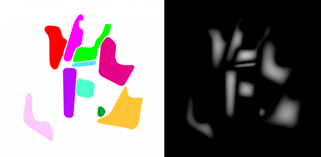
To calculate the terrain and elevate each each area on the map we use two different images (see below) One image has all the areas mapped with different colours and the other image is the height map which uses only two colours, black and white, white colour represents a higher elevation. Combining these two images, the map image, the data about each area and the shaders we were able to develop the interactive Map for Loom Atlas.
Challenges
Creating curvature in the terrains
To calculate the elevation (curvature) of the terrains we use the height map image (black and white). After 30 different prototypes testing all sort of properties like number of segments, colours, opacity, dimensions, camera positions, transitions, data relations the most challenging part was to combine all the shaders calculations with the data and achieve a nice and smooth map interaction.
The current map uses 64 segments on top terrain and 64 segments on bottom terrain. So each terrain has 4425 vertices, but only vertices inside one of the 12 areas on the map will be calculated.
A shader is a small program written in GLSL to run on the GPU (Graphic Processing Unit).
Calculating the sub terrains
There were some algorithmic challenges faced when looking at comparing the digitised vs non-digitised data within Atlas. The elevations on glance needed to highlight to the user just how much has been digitised within the libraries collections. But the data various so much across time and location, that we needed to develop an algorithm that found the middle ground between all the data across all locations.
Using the numbers for digitised and non-digitised records for each area per gap of year, the top elevation is based on the average of digitised counts across all areas. The bottom elevation is based on each area top elevation so if one area has 200 digitised and 40 non-digitised records the top elevation height is 100 so the bottom elevation height will be 20 ( 20% of the top height).